
Inter-Subject Correlation Analysis in Music-Induced EEG Responses
Published:
An exploration of neural synchronization patterns in participants with varying levels of agreement on musical preferences, conducted as part of an independent study with the IIIT-H Music Cognition Group with the support and guidance of Prof. Vinoo Alluri.
Introduction
This independent study investigates how inter-subject correlation (ISC) in EEG responses varies between groups of participants who agree versus disagree on their subjective ratings of music. Using the DEAP dataset, we identified participant groups with high and low agreement on valence and liking ratings, then analyzed their neural synchronization patterns across different frequency bands and brain regions.
Part 1: Exploratory Data Analysis
Dataset Overview
The DEAP (Database for Emotion Analysis using Physiological signals) dataset provided the foundation for this study:
- 40 music videos (63 seconds each)
- 32 participants
- EEG recorded at 128 Hz → 8,064 timepoints per song
- 32 EEG channels categorized into 10 functional brain regions
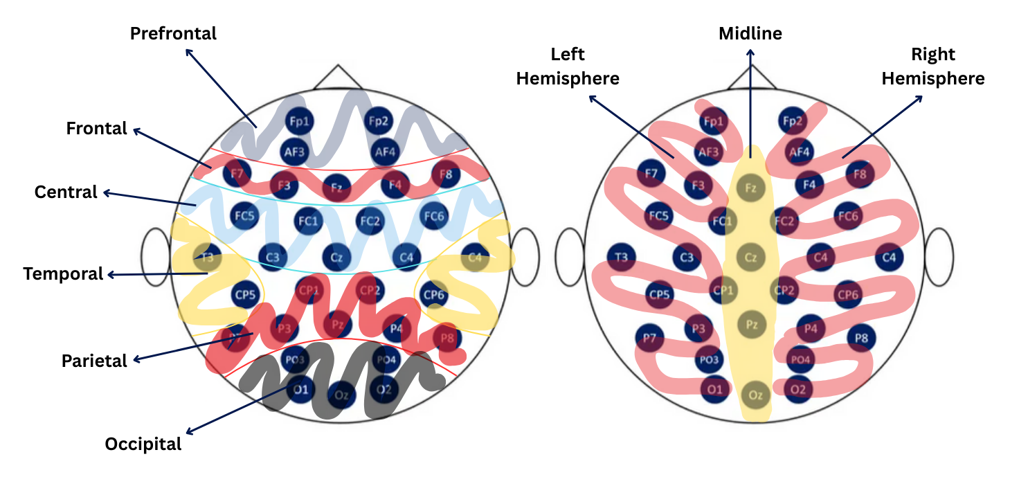
Brain Region Classification
The 32 EEG channels were organized into the following regions:
region_dict = {
    "Prefrontal": [1, 17, 2, 18],        # Fp1, Fp2, AF3, AF4
    "Frontal": [3, 20, 4, 21, 19],       # F3, F4, F7, F8, Fz
    "Central": [6, 23, 5, 22, 7, 25, 24], # FC1, FC2, FC5, FC6, C3, C4, Cz
    "Temporal": [8, 26, 9, 27],          # T7, T8, CP5, CP6
    "Parietal": [11, 29, 12, 30, 16, 10, 28], # P3, P4, P7, P8, Pz, CP1, CP2
    "Occipital": [14, 32, 15, 13, 31],   # O1, O2, Oz, PO3, PO4
    "LeftHemisphere": [1, 2, 3, 4, 5, 6, 7, 8, 9, 10, 11, 12, 13, 14],
    "RightHemisphere": [17, 18, 20, 21, 22, 23, 25, 26, 27, 28, 29, 30, 31, 32],
    "Midline": [15, 16, 19, 24],         # Oz, Pz, Fz, Cz
    "Global": list(range(1, 33))         # All electrodes
}
Subjective Ratings
Each participant rated all 40 songs on four dimensions (scale 1-9):
- Valence (negative to positive emotion)
- Arousal (calm to excited)
- Dominance (submissive to dominant)
- Liking (dislike to like)
For this study, we focused on Valence and Liking as the primary indicators of musical preference.
Correlation Analysis
Initial correlation matrices revealed participant-by-participant agreement patterns:
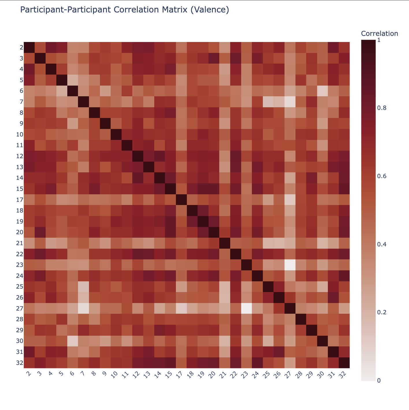
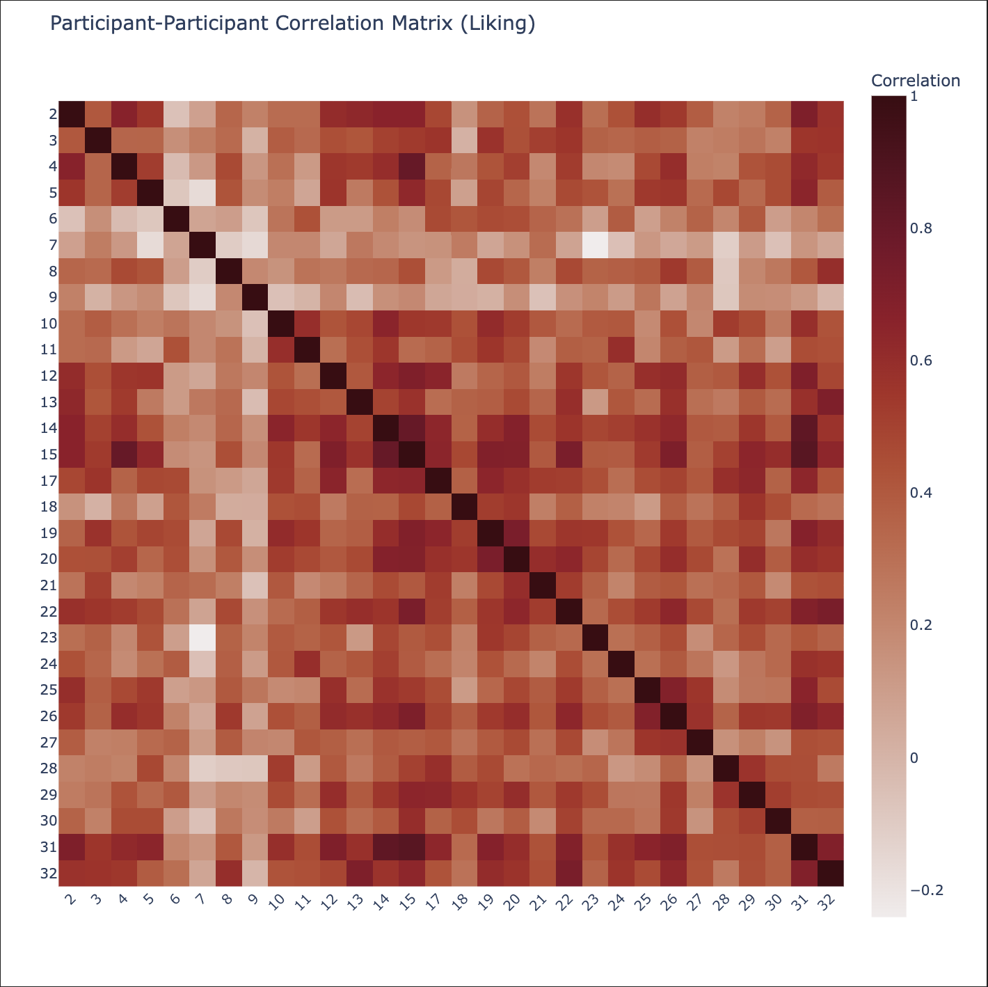
Key Finding: Participants 1 and 16 showed extremely low correlations with others and were excluded as outliers from subsequent analyses.
Computing Agreement and Disagreement Groups
Graph Theory Approach
Using graph theory and clique detection, we identified groups of participants with high mutual agreement and low mutual agreement on musical preferences.
Agreement Group Selection
Methodology:
- Constructed a graph where:
- Nodes = participants
- Edges = participants with correlation ≥ 0.6 (valence) AND ≥ 0.5 (liking)
- Identified cliques (fully connected subgraphs) with minimum 3 participants
- Ranked cliques by scoring system:
Best Agreement Clique:
- Participants: 14, 15, 19, 20, 22, 32
- Average Score: 0.723
- Group Size: 6 participants
Disagreement Group Selection
An exhaustive search on the remaining 24 participants (excluding outliers 1, 16 and the 6 agreement participants) identified the group with the lowest mutual correlation scores.
Worst Disagreement Group:
- Participants: 6, 7, 9, 23, 27, 30
- Average Score: 0.193
- Group Size: 6 participants
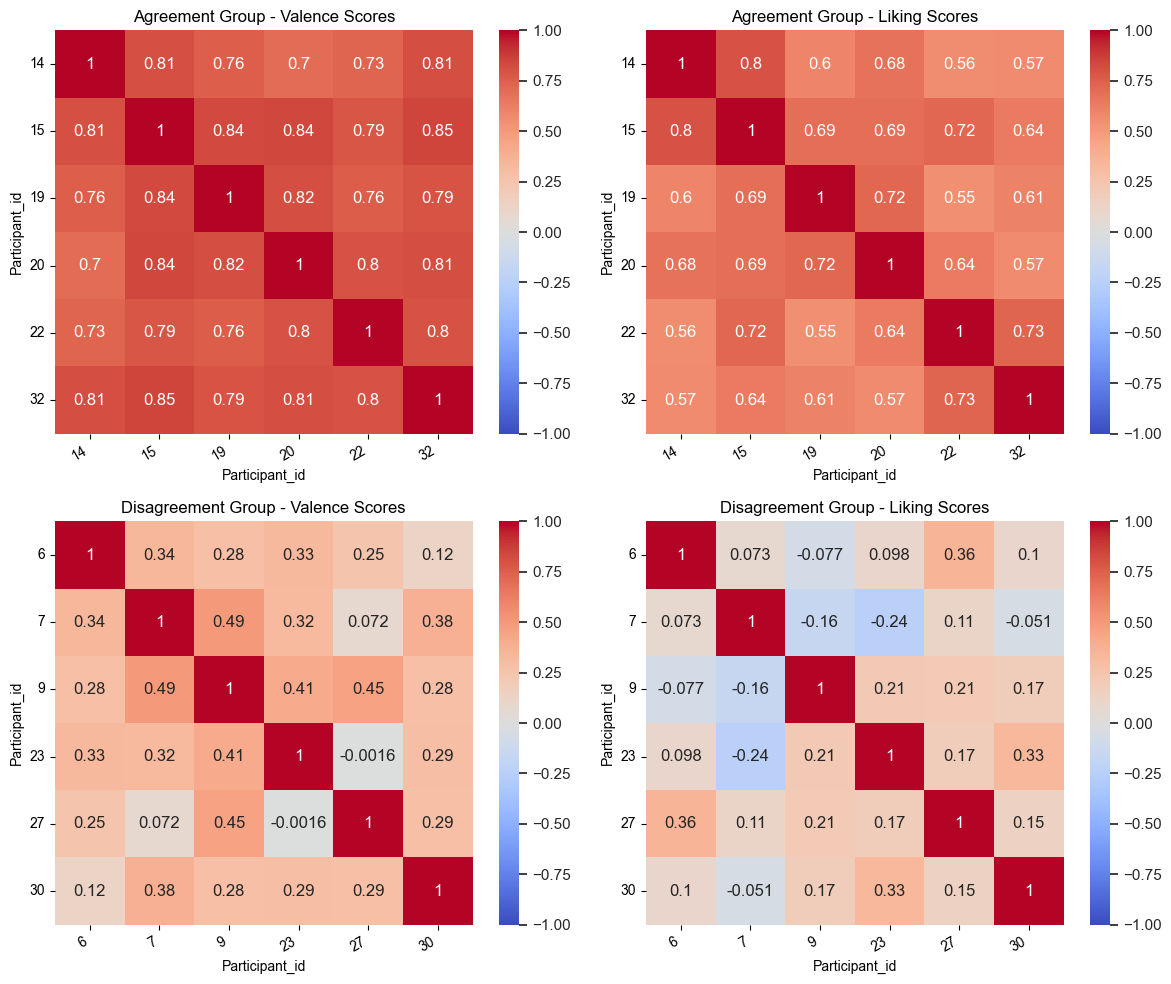
Group Validation
The two groups showed clear separation in their correlation patterns:
| Metric | Agreement Group | Disagreement Group |
|---|---|---|
| Valence Score | 0.794 | 0.288 |
| Liking Score | 0.651 | 0.097 |
| Average Score | 0.723 | 0.193 |
Part 2: Inter-Subject Correlation (ISC) Computation
Methodology Overview
The ISC computation pipeline consisted of the following steps:
- Load EEG data for specific song, group, frequency band, and region
- Compute spectral power using Welch’s method
- Create correlation matrices between participants
- Calculate ISC statistics (min, max, mean, std)
Frequency Bands of Interest
freq_band_dict = {
    "Theta": (4, 8),      # Associated with memory and emotion
    "Alpha": (8, 13),     # Associated with attention and relaxation
    "Beta": (13, 30),     # Associated with active thinking
    "Gamma": (30, 45),    # Associated with cognitive processing
    "All": (4, 45)        # Broadband analysis
}
Data Preprocessing Challenges
Challenge 1: Electrode Labeling Inconsistency
Problem: Participants 1-22 used Twente channel ordering, while participants 23-32 used Geneva ordering.
Solution: Applied mapping table to convert all data to Geneva format for consistency.
Challenge 2: Trial Order Randomization
Problem: Each participant experienced the 40 songs in a different random order.
Solution: Used the Experiment_id column in participant_ratings.csv to correctly map trial numbers to song identities for each participant.
Spectral Power Estimation: Welch’s Method
What is Welch’s Method?
Welch’s method estimates the power spectral density (PSD) of a signal by:
- Splitting the signal into overlapping windows
- Applying a windowing function (Hamming) to each segment
- Computing periodograms (FFT-based power estimates) for each window
- Averaging periodograms to reduce noise
Parameters Used:
- Sampling rate: 128 Hz
- Signal duration: 63 seconds (8,064 timepoints)
- Window size: 2 seconds (256 samples)
- Hop length: 0.5 seconds (64 samples)
- Result: 123 windows per recording
ISC Calculation Process
For each combination of (song, region, frequency band, group):
- Load and filter EEG:
- Extract relevant channels for the brain region
- Apply bandpass filter for frequency band
- Stack across participants:
(n_channels, n_timepoints, n_participants)
- Compute spectral power:
- Apply Welch’s method per channel and participant
- Result:
(n_channels, 123 windows, n_participants)
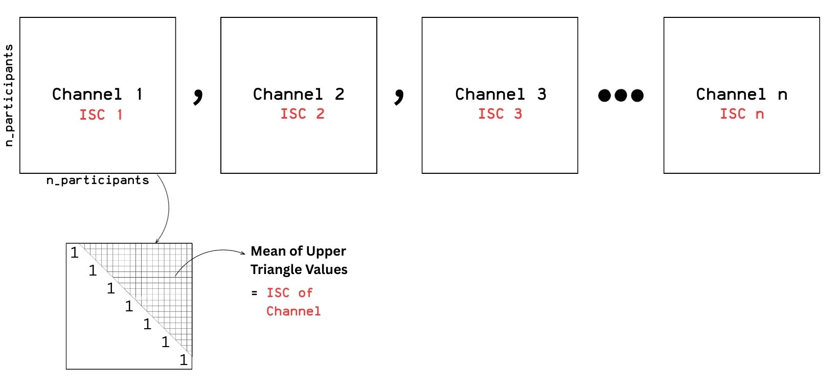
- Create correlation matrices:
- For each channel, compute pairwise Pearson correlations between all participant PSD time series
- Result:
(n_participants × n_participants)matrix per channel
- Extract ISC values:
- Take upper triangle of correlation matrix (excluding diagonal)
- Compute statistics: min ISC, max ISC, mean ISC, std ISC
Computational Scope
Total combinations analyzed: 4,000
- 40 songs × 10 regions × 5 frequency bands × 2 groups = 4,000
Each combination produced one row in the output CSV:
Group, Song_Index, Frequency_Band, Region, Mean_ISC, Min_ISC, Max_ISC, Std_ISC
Part 3: Statistical Analysis of ISC
Analysis Framework
The mean ISC values from 4,000 combinations were aggregated for statistical testing:
- Statistical unit: mean ISC (origin-independent)
- Frequency bands: 5 (Theta, Alpha, Beta, Gamma, All)
- Brain regions: 10
- Analysis combinations: 50 (5 bands × 10 regions)
- Sample size per combination: 40 (one per song) for each group
Independent T-Tests
Hypothesis:
- Null (H₀): Agreement group ISC mean = Disagreement group ISC mean
- Alternative (H₁): The means of the two groups differ (two-tailed)
T-statistic formula:
\[t = \frac{\bar{X}_1 - \bar{X}_2}{\sqrt{\frac{s_1^2}{n_1} + \frac{s_2^2}{n_2}}}\]Where:
- $\bar{X}_1, \bar{X}_2$ = sample means
- $s_1^2, s_2^2$ = sample variances
- $n_1, n_2$ = sample sizes (both = 40)
Degrees of freedom (Welch-Satterthwaite equation):
\[df = \frac{\left(\frac{s_1^2}{n_1} + \frac{s_2^2}{n_2}\right)^2}{\frac{(s_1^2/n_1)^2}{n_1-1} + \frac{(s_2^2/n_2)^2}{n_2-1}}\]Results: 24 out of 50 combinations showed significant differences (p < 0.05)
Effect Size: Cohen’s d
Why effect size matters:
While p-values indicate whether an effect exists, Cohen’s d quantifies how large that effect is—crucial for interpreting practical significance in neuroscience.
Calculation:
For equal-sized groups, Cohen’s d can be approximated from the t-statistic:
\[d = \frac{t}{\sqrt{n}}\]Where t = t-statistic and n = 40 (observations per group)
Interpretation guidelines:
| Cohen’s d | Effect Strength |
|---|---|
| < 0.2 | Trivial |
| 0.2 - 0.5 | Small |
| 0.5 - 0.8 | Moderate |
| > 0.8 | Large |
Key Findings from Effect Size Analysis
Top 5 Highest Effect Sizes:
| Band | Region | Cohen’s d | Effect Strength |
|---|---|---|---|
| Alpha | Prefrontal | 0.550 | Moderate |
| Alpha | Frontal | 0.519 | Moderate |
| Alpha | Left Hemisphere | 0.502 | Moderate |
| Alpha | Parietal | 0.483 | Small-Moderate |
| Alpha | Global | 0.477 | Small-Moderate |
Key Insights:
- Most differences showed small effects (d = 0.2-0.5), typical in naturalistic EEG with high variability
- Moderate effects (d ≥ 0.5) appeared exclusively in the Alpha band, particularly over frontal regions
- Alpha-band ISC appears most sensitive to shared cognitive states related to attention and engagement
Statistical Power Analysis
What is statistical power?
Power is the probability of detecting a true effect when it exists (correctly rejecting H₀). It depends on:
- Effect size (Cohen’s d)
- Sample size (n = 40 per group)
- Significance level (α = 0.05)
Power calculation:
\[\text{Power} = 1 - \beta\]where β = probability of Type II error
Computed using TTestIndPower from statsmodels based on Cohen’s d, sample size, and α = 0.05 (two-tailed).
Top 5 Highest Power Values:
| Band | Region | Cohen’s d | Statistical Power |
|---|---|---|---|
| Alpha | Prefrontal | 0.550 | 0.680 |
| Alpha | Frontal | 0.519 | 0.631 |
| Alpha | Left Hemisphere | 0.502 | 0.601 |
| Alpha | Parietal | 0.483 | 0.568 |
| Alpha | Global | 0.477 | 0.559 |
Key Insights:
- Moderate power (0.3-0.6) for most tests—expected given small-to-medium effect sizes
- Highest power in Alpha band (>0.6 for Prefrontal, Frontal, Left Hemisphere)
- Lowest power in some Theta and All-band combinations (<0.3), indicating marginal detectability
Complete Results: 24 Significant Combinations
Theta Band (7 significant regions):
| Region | Agreement Mean | Disagreement Mean | t-statistic | p-value | Cohen’s d | Power |
|---|---|---|---|---|---|---|
| Frontal | 0.0278 | 0.0099 | 2.192 | 0.032 | 0.347 | 0.334 |
| Central | 0.0258 | 0.0094 | 2.311 | 0.024 | 0.365 | 0.365 |
| Parietal | 0.0307 | 0.0112 | 2.419 | 0.018 | 0.383 | 0.394 |
| Occipital | 0.0300 | 0.0102 | 2.435 | 0.017 | 0.385 | 0.398 |
| Left Hemisphere | 0.0290 | 0.0108 | 2.387 | 0.020 | 0.377 | 0.385 |
| Midline | 0.0225 | 0.0074 | 2.062 | 0.043 | 0.326 | 0.302 |
| Global | 0.0283 | 0.0115 | 2.197 | 0.031 | 0.347 | 0.335 |
Alpha Band (9 significant regions):
| Region | Agreement Mean | Disagreement Mean | t-statistic | p-value | Cohen’s d | Power |
|---|---|---|---|---|---|---|
| Prefrontal | 0.0336 | 0.0148 | 3.476 | 0.001 | 0.550 | 0.680 |
| Frontal | 0.0284 | 0.0084 | 3.285 | 0.002 | 0.519 | 0.631 |
| Central | 0.0214 | 0.0085 | 2.197 | 0.031 | 0.347 | 0.335 |
| Parietal | 0.0232 | 0.0047 | 3.052 | 0.003 | 0.483 | 0.568 |
| Occipital | 0.0268 | 0.0107 | 2.522 | 0.014 | 0.399 | 0.421 |
| Left Hemisphere | 0.0247 | 0.0066 | 3.174 | 0.002 | 0.502 | 0.601 |
| Right Hemisphere | 0.0246 | 0.0097 | 2.615 | 0.011 | 0.413 | 0.447 |
| Midline | 0.0276 | 0.0107 | 2.812 | 0.006 | 0.445 | 0.501 |
| Global | 0.0250 | 0.0085 | 3.020 | 0.004 | 0.477 | 0.559 |
All Band (8 significant regions):
| Region | Agreement Mean | Disagreement Mean | t-statistic | p-value | Cohen’s d | Power |
|---|---|---|---|---|---|---|
| Prefrontal | 0.0350 | 0.0194 | 2.147 | 0.035 | 0.340 | 0.323 |
| Frontal | 0.0351 | 0.0160 | 2.348 | 0.022 | 0.371 | 0.375 |
| Global | 0.0322 | 0.0146 | 2.368 | 0.021 | 0.374 | 0.380 |
| Right Hemisphere | 0.0338 | 0.0175 | 2.097 | 0.040 | 0.332 | 0.310 |
| Left Hemisphere | 0.0322 | 0.0121 | 2.674 | 0.009 | 0.423 | 0.463 |
| Occipital | 0.0320 | 0.0137 | 2.352 | 0.021 | 0.372 | 0.376 |
| Parietal | 0.0336 | 0.0135 | 2.536 | 0.013 | 0.401 | 0.425 |
| Central | 0.0283 | 0.0127 | 2.110 | 0.038 | 0.334 | 0.314 |
Part 4: Complementary Per-Channel ISC Analysis
Motivation for Channel-Level Analysis
While region-based ISC (Part 2) provided broad insights into brain area differences, it masked finer spatial variations within regions. The per-channel approach offers:
- Higher spatial resolution: ISC computed for each of 32 electrodes independently
- Visual interpretability: Results visualized on topographic scalp maps
- Consistency verification: Identifies which specific electrodes drive regional effects
Computation Methodology
Input format: For each (Group, Song, Frequency Band) combination:
- EEG shape:
(32 channels, 8064 timepoints, 6 participants) - All 32 electrodes loaded per participant (no regional grouping)
- Same spectral power and ISC computation as Part 2, but per individual channel
Output structure:
Group, Song_Index, Frequency_Band, ISC1, ISC2, ..., ISC32
- One row per combination
- Total rows: 2 groups × 40 songs × 5 bands = 400
- Each ISC_i = mean ISC for channel i across all participant pairs
Topographic Visualization
To interpret spatial patterns of ISC differences:
- Average ISC per channel across all 40 songs for each group and frequency band
- Plot on scalp using MNE’s topomap visualization (biosemi32 montage)
- Compare Agreement vs. Disagreement groups side-by-side
Benefits:
- Provides spatial context to statistical results from Part 3
- If “Parietal-Alpha” was significant in region-based analysis, topomaps show which parietal electrodes drove the effect
- Reveals gradients and hotspots of neural synchronization
Part 5: Comprehensive Visualizations
Heatmap: T-Test Results Across All Combinations
This heatmap displays the difference in mean ISC between Agreement and Disagreement groups for all 50 (Region × Band) combinations:
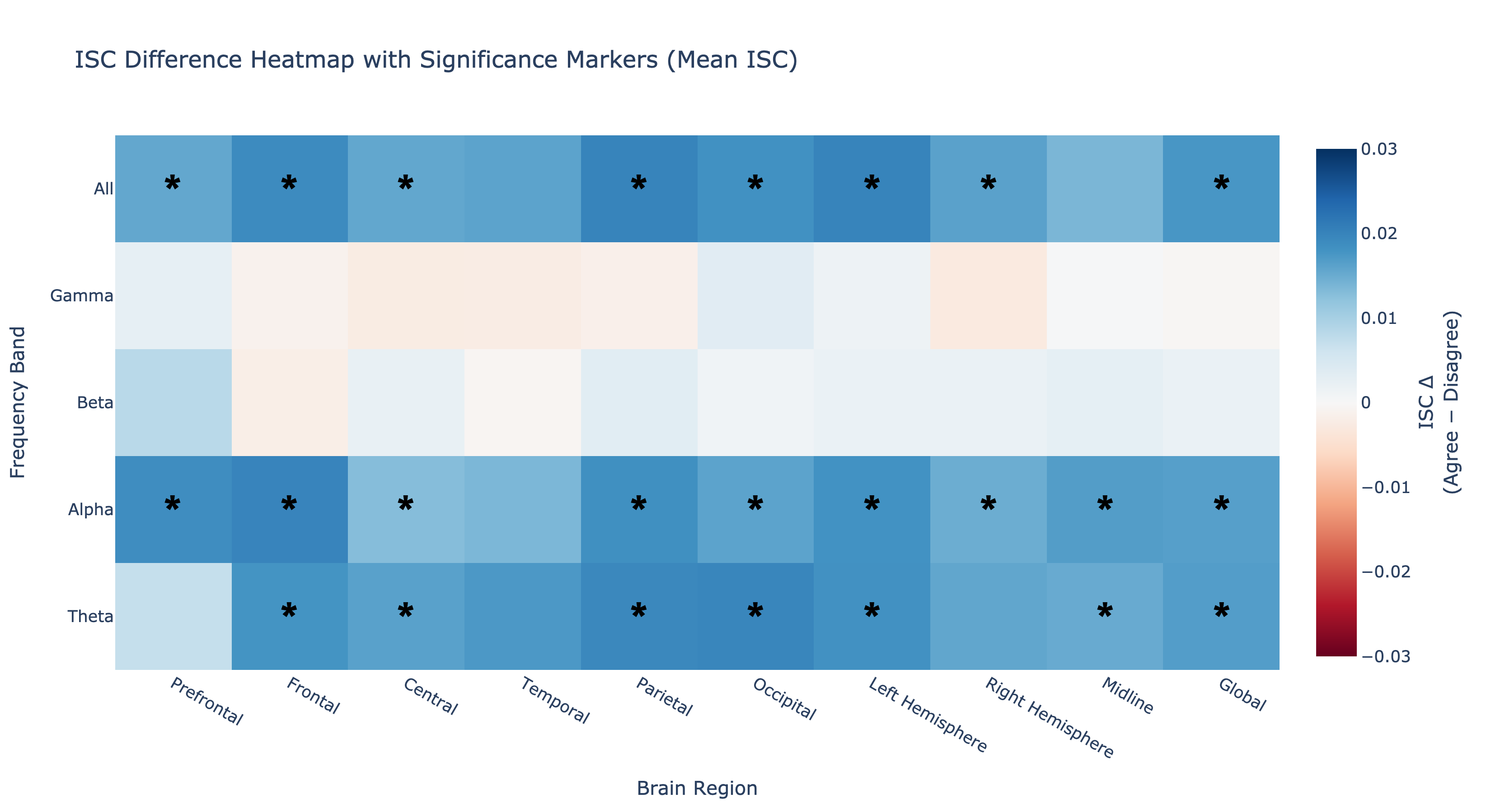
Legend:
- Color intensity = magnitude of ISC difference (Agreement - Disagreement)
*denotes statistically significant p-value (p < 0.05)- Difference in means is directly proportional to Cohen’s d (effect size)
Key Observations:
- Alpha band shows the most widespread and strongest differences
- Prefrontal, Frontal, and Left Hemisphere regions exhibit largest effects
- Beta and Gamma bands show minimal differences
Topographic Maps: Alpha Band Comparison
The Alpha band was the only frequency range with consistently significant combinations showing moderate effect sizes and statistical power. Below are comparative topomaps for Agreement vs. Disagreement groups:
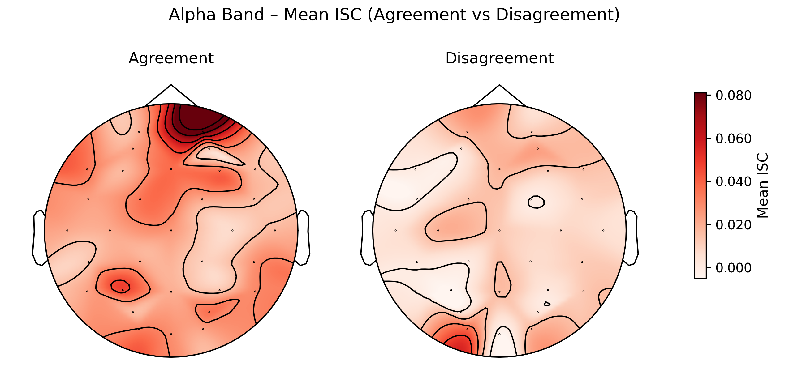
Visual Insights:
- Agreement group shows higher ISC across frontal and parietal regions
- Particularly pronounced in prefrontal (Fp1, Fp2, AF3, AF4) and frontal (F3, F4, Fz) electrodes
- Disagreement group shows more uniform, lower ISC across the scalp
- Spatial pattern confirms region-based statistical findings
Final Interpretations
Statistical Summary
1. Alpha Band Dominance
Finding: The Alpha band (8-13 Hz) showed the strongest and most consistent differences between agreement and disagreement groups across nearly all brain regions.
Evidence:
- Highly significant p-values across all regions (all p < 0.05, most p < 0.01)
- Largest effect sizes of any frequency band
- Highest statistical power (up to 0.68 for Prefrontal)
| Region | Cohen’s d | Effect Strength | Statistical Power |
|---|---|---|---|
| Prefrontal | 0.550 | Moderate | 0.680 |
| Frontal | 0.519 | Moderate | 0.631 |
| Left Hemisphere | 0.502 | Moderate | 0.601 |
| Parietal | 0.483 | Small-Moderate | 0.568 |
| Global | 0.477 | Small-Moderate | 0.559 |
2. Small but Meaningful Effects
Finding: Most group differences showed small effects (Cohen’s d = 0.2-0.5), which is expected and appropriate in naturalistic EEG settings.
Interpretation:
- High inter-individual variability is inherent in real-world neural data
- Small effects can still be meaningful when consistently observed across multiple conditions
- Moderate effects in Alpha band suggest this frequency range is particularly sensitive to shared cognitive states
3. Spatial Patterns
Finding: Moderate effects were concentrated in frontal and parietal regions, with strong left hemisphere involvement.
Topographic confirmation:
- Agreement group participants showed elevated ISC particularly in prefrontal (Fp1, Fp2, AF3, AF4) and frontal (F3, F4, Fz) electrodes
- Spatial gradient visible from front to back, with strongest effects anteriorly
- Consistent with region-based statistical tests
Cognitive Interpretations
While formal cognitive conclusions require further validation, these patterns suggest several plausible interpretations:
Alpha Oscillations and Attention
Alpha-band activity (8-13 Hz) is strongly associated with:
- Attention allocation and selective inhibition
- Working memory maintenance
- Top-down cognitive control
Implication: Participants who agree on musical preferences may exhibit more similar patterns of attention deployment and cognitive engagement during listening.
Frontal Involvement
Prefrontal and frontal regions are critical for:
- Aesthetic judgment and preference formation
- Emotional evaluation
- Executive control during music listening
Implication: Neural synchronization in these regions may reflect shared evaluative processes and emotional responses to music.
Left Hemisphere Lateralization
Left-hemisphere dominance in the observed effects may relate to:
- Temporal processing and rhythm perception
- Language-like analytical processing of music
- Positive emotional valence (left-frontal approach motivation)
Implication: Agreement on musical preferences may involve similar left-lateralized cognitive strategies for music processing.
Methodological Strengths
- Robust group identification: Graph-theoretic clique detection ensured maximal within-group agreement and between-group separation
- Comprehensive frequency analysis: Five frequency bands provided complete spectral coverage
- Multiple spatial scales: Both region-based and per-channel analyses offered complementary insights
- Rigorous statistics: Effect sizes and power analyses contextualized significance tests
- Visual validation: Topographic maps provided intuitive spatial confirmation of statistical results
Limitations and Future Directions
Current limitations:
- Sample size (n=6 per group) limited by strict agreement/disagreement criteria
- Cross-sectional design prevents causal inference
- Musical stimuli varied in genre, tempo, and structure
Future research could:
- Expand to larger participant pools with varied musical backgrounds
- Control for specific musical features (tempo, key, complexity)
- Investigate other frequency bands (Beta, Gamma) with targeted hypotheses
- Explore directed connectivity measures (e.g., Granger causality)
- Incorporate behavioral measures of engagement and attention
Conclusion
This study demonstrated that inter-subject correlation in Alpha-band EEG activity differs significantly between groups with high versus low agreement on musical preferences, particularly in prefrontal, frontal, and parietal regions. These findings suggest that shared musical preferences may be associated with similar patterns of neural synchronization during listening, potentially reflecting common cognitive and emotional processing strategies.
The Alpha band’s unique sensitivity to these group differences highlights the importance of attentional and evaluative processes in shaping individual music preferences. Future work combining neural, behavioral, and computational approaches will be essential for fully understanding the complex relationship between brain activity and musical experience.
Acknowledgments
This work was conducted as part of an independent study with the IIIT-Hyderabad Music Cognition Group under the guidance of Prof. Vinoo Alluri. I am deeply grateful to Prof. Alluri for her invaluable support, insights, and mentorship throughout this project, and to the members of the Music Cognition Group for their feedback and encouragement.
Technical Implementation
Tools and Libraries:
- Python 3.x for all analyses
- NumPy & SciPy for signal processing
- Pandas for data manipulation
- MNE-Python for EEG visualization
- Statsmodels for statistical testing
- Matplotlib & Seaborn for visualization
- NetworkX for graph-theoretic clique detection
Dataset:
- DEAP (Database for Emotion Analysis using Physiological signals)
- Available at: http://www.eecs.qmul.ac.uk/mmv/datasets/deap/
For questions or collaboration opportunities, feel free to reach out.